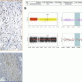
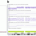
Bioinformatics for Precision Medicine in Oncology

Fig. 6.1

Framework for PM in oncology. The left part describes the workflow and processes required for the decision-making from patient consultation to the therapeutic decision. The middle part focuses on the informatics and bioinformatics architecture required to support the different steps of the workflow. The right part indicates the different experts involved in each process

6.1.2 Need for Bioinformatics Solutions to Support Precision Medicine

The availability of high-throughput technologies dedicated to clinical applications makes it very attractive for cancer centers to use these new tools on a daily basis. However, establishing such a clinical facility is not a trivial task due to the aforementioned complexity of PM framework along with the overwhelming amount of data. Indeed, the field of oncology has entered the so-called big data era as the particle physics did several years ago. From the big data 4 V’s perspective, data integration issue (i.e., merging heterogeneous data in a seamless information system) in oncology can be formulated as follows: a large volume of patients’ data is disseminated across a large variety of databases which increase in size at a huge velocity. In order to extract most of the hidden value from these data, we must face challenges at (1) the technical level to develop a powerful computational architecture (software/hardware); (2) the organizational and management levels to define the procedures to collect data with highest confidence, quality, and traceability; and (3) the scientific level to create sophisticated mathematical models to predict the evolution of the disease and risks to the patient. Obviously, an efficient informatics and bioinformatics architecture is definitely needed to support PM in order to record, manage, and analyze all the information collected. The architecture must also permit the query and the easy retrieval of any data that might be useful for therapeutic decision in real time, thus allowing clinicians to propose the tailored therapy to the patient in the shortest delay. Therefore, bioinformatics is among the most important bottlenecks toward the routine application of PM, and several challenges need to be faced to make it a reality (Fernald et al. 2011). First, the development of a seamless information system allowing data integration, data traceability, and knowledge sharing across the different stakeholders is mandatory. Second, bioinformatics pipelines need to be developed in order to provide relevant biological information from the high-throughput molecular profiles of the patient. Third, the architecture must warrant the reproducibility of the results.

If many recent publications point out the key role of the bioinformatics for PM today (Simon and Roychowdhury 2013), clinical trials usually do not detail the complete bioinformatics environment used in practice to assess the quality and the traceability of the generated data. Different software platforms such as tranSMART (Athey et al. 2013), G-DOC (Madhavan et al. 2011) or the cBioPortal for Cancer Genomics (Cerami et al. 2012) have been recently developed to promote the data sharing and analysis of genomics data in translational research. Canuel et al. (2014) reviewed the different solutions available and compared their functionalities. One of the most interesting features of these platforms relies on their analytical functionalities. They provide ready-to-use tools through user-friendly interface offering interesting functionalities for data queries and user analysis. However, these different solutions do not address essential aspects which are offered by our system: first, often they handle a specific type of data; second, they do not cover management and traceability of the data in real time as long as they are generated by the different stakeholders; and third, they do not provide clinicians with a meaningful digest of the analyses, which they need to take clinical decisions.

6.1.3 Seamless Information System

Precision medicine relies on a tight connection between many different stakeholders. As the choice of the therapy is based on a combination of different information levels including clinical data, high-throughput profiles (somatic mutations and DNA copy number alterations), and IHC data, all this information related to a given patient needs to be gathered in a seamless information system. Data integration is definitely required, and bioinformatics plays a central role in setting up this infrastructure. The information system must ensure data sharing, cross software interoperability, automatic data extraction, and secure data transfer. In the context of the SHIVA clinical trial, high-throughput and IHC data are sent by the different biotechnological platforms to the bioinformatics platform using standardized procedures for transfer and synchronization. Data are then integrated into the information system within ad hoc repositories and databases. Metadata describing the data are stored in the core database such as the patient identifier, the type of data (e.g., mutation screening, clinical data, DNA copy number profile), and the technology used (e.g., Affymetrix microarray, Ion Torrent^™ PGM sequencing). Each type of data is then processed by dedicated bioinformatics pipelines in order to extract the relevant biological information such as the list of mutations and the list of amplifications/deletions. Therefore, the core database of the system acts as a hub allowing referencing all data through the use of web services. It knows exhaustively which data is available for a given patient and where the raw and processed data are physically stored. It thus offers the possibility for clinicians to make queries through a web application and to extract the list of available information for a given patient. In addition, the system is also used to manage and perform automatic integrative analysis required for the therapeutic decision.

6.2 High-Throughput Data Analyses and Reporting

The DNA copy number analysis is now well defined, following standard analysis workflow. Many other books or papers already present in details this application. For this reason, the current section is mainly dedicated to NGS data analysis.

6.2.1 DNA Copy Number Analysis

The use of DNA copy number microarray allows both the detection of DNA copy number alterations and the loss of heterozygosity events. As an example, we will illustrate the analysis of Affymetrix microarray data.

Raw data are usually normalized with the Affymetrix Power Tools software package (http://www.affymetrix.com) in order to remove systematic and technological bias. Then, the log R ratio is segmented in order to detect breakpoints and assign copy number status (Rigaill 2010; Hupé et al. 2004). A similar process is applied on the allele difference profile as performed by the GAP software (Popova et al. 2009). Both profiles (DNA copy number and LOH) allow the estimation of absolute copy number for each probe taking into account the sample cellularity and tumor ploidy.

Each gene status (normal, gained, amplified, lost, deleted, loss of heterozygosity) can then be assessed. Copy number alterations are defined as follows: deletion = 0 copy; loss = 1 copy; normal = 2 copies; gain = 3, 4, or 5 copies; and amplification ≥6 copies for diploid tumor and deletion = 0 copy; loss = 1 or 2 copies; normal = 3 or 4 copies; gain = 5 or 6 copies; and amplification ≥7 copies for tetraploid tumors.

Additional steps in the analysis can be performed to distinguish between large-scale events such as chromosome arm gain and focal events targeting single oncogene or tumor-suppressor gene. Focal gains and amplifications are defined as genomic alterations with a size less than 10 Mb and a copy number greater than the surrounding regions. In order to check whether a focal gain or an amplification of a size between 1 and 10 Mb induces a protein overexpression, a validation using IHC can be applied for clinical decision.

6.2.2 Analysis of High-Throughput Sequencing and Clinical Applications

6.2.2.1 General Principles of High-Throughput Sequencing Analysis

The next-generation sequencing (NGS) technologies have emerged around 2008 and have exploded a few years later. First used in research projects, they rapidly pave the way to new clinical applications. Today, the NGS technologies have almost no limitation in terms of biological applications and continue to evolve very rapidly. NGS offers the possibility to sequence a full human genome in less than two weeks for a few thousand dollars where 2.7 billions dollars and more than 10 years were required by the Human Genome Project to deliver the first human genome draft in 2001. In early 2004, the second generation of sequencers provided an increase of the throughput capacity with a lower cost and is today widely used both in research and clinical screenings. NGS technologies are a very competitive field and third (single molecule) and fourth generations (nanopore technologies) of sequencers are already available or under development.

The biological applications of NGS can be broadly classified in three main classes according to their biological context: the DNA world, the RNA world, and the epigenetic world, each of them being subdivided in several sequencing techniques and methodological workflows. If the use of RNA sequencing starts to emerge as a diagnosis tool, the DNA sequencing remains the main application for clinics. In addition to whole-genome sequencing, target-enrichment methods have been developed to selectively capture genomic regions of interest from a DNA sample prior to sequencing. The exome sequencing consists of selecting only the subset of DNA coding regions before sequencing. Other targeted strategies can be defined at the gene or amplicon levels, making these applications cost-effective for a large number of samples.

The analysis of these data has been an important bioinformatics challenge of the recent years. The main difficulty in comparison with the microarray analyses comes from the size of the data to manipulate. Thus, if microarray analysis can be performed today on a single laptop, analyzing a large NGS dataset requires a dedicated computational infrastructure as well as strong computational skills. Once the targeted DNA region is sequenced, the first steps of the analysis are usually common to many different types of sequencing applications (quality control, cleaning, reads alignment). Then, the secondary analysis aims at answering a dedicated biological question. In oncology, this question is usually to detect with high sensibility and specificity somatic mutations. But other questions such as detection of copy number variants or large rearrangements can also be addressed using NGS techniques. In the following part, we will describe in details each step of the analysis, from the raw reads to the list of filtered variants used by the clinicians for therapeutical decision.

6.2.2.2 Definition and Key Concepts

Before presenting the different steps of a sequencing analysis project, key notions and vocabulary common to all applications have to be defined. The reads refer to the sequences called and delivered by the sequencing machine. These reads are associated with quality values describing the probability of a given call to be a sequencing error (see Sect. 6.2.2.3 for details). The first question which usually comes when a project is designed is about the number of reads required to answer the biological question. Whereas the recent technologies are able to produce billion of reads per flow cell, most of the applications only require a few dozen (or hundred) millions of reads per sample, thus allowing the multiplexing of several samples using different barcodes. The number of reads required per sample depends on the sequencing depth, which is the average number of reads spanning one nucleotide. For instance, the current sequencing depth advised to detect with a good accuracy a germline variant is around 30X. It means that a homozygous variant should be supported in average by 30 reads (15 for each allele in the case of a heterozygous variant). In the case of somatic mutations and cancer samples, the higher will be the sequencing depth, and the lower will be the detection threshold at which a variant may be called. For instance, with a sequencing depth of 100X, a variant with a frequency of 10 % will be supported by only ten reads. Note that it is important to differentiate the sequencing depth from the coverage. The latter represents the fraction of the genome which is supported by at least one read (Fig. 6.2).

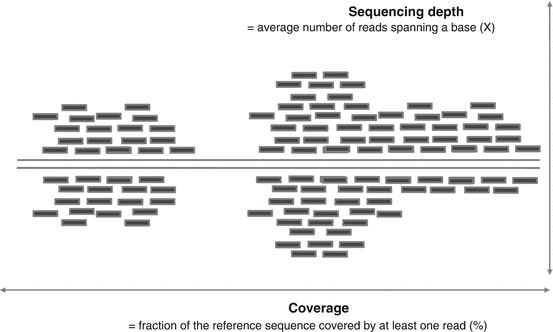
Fig. 6.2

Sequencing depth versus coverage. The sequencing depth is defined as the mean number of reads covering one base, whereas the coverage represents the fraction of the genome which is read at least once

6.2.2.3 Quality Control of Sequencing Reads

Any high-throughput technology, even if well standardized, suffers from experimental bias. Adequate experimental designs and good laboratory practice are thus mandatory to limit the variation among samples. This point is even more true in clinical practice where the reliability of high-throughput screening is expected to be higher. Therefore, a quality control procedure needs to be defined.

The FASTQ format is a standard text-based format for storing both the nucleotide sequence and its corresponding quality scores. Both the nucleotide and the quality score at each position are encoded as ASCII character. The quality values are encoded as Phred scores Q and are logarithmically related to the base-calling error probabilities P (1):

$Q=-10\; \log 10\;P\;(1)$

For instance, a Phred quality score of 20 (Q20) assigned to a base means that the probability of an incorrect base call is 1–100 times (Table 6.1). It means that the base call accuracy is 99 % and that every 100 bp, a sequencing read will likely contain an error.

Table 6.1

Phred quality value

Phred quality score	Error probability	Base accuracy (%)
10	1 in 10	90
20	1 in 100	99
30	1 in 1000	99.9
40	1 in 10,000	99.99

The sequencing quality values are encoded as Phred scores and are logarithmically related to the base-calling error probabilities. A minimum quality score of 20 is usually used to select high confidence data.

Starting from the raw reads from the sequencers, several quality controls can be applied:

Sequence quality. One standard way of representing the reads quality is to display the range of quality values across all bases at each position in the FASTQ file. The first nucleotides of the reads usually have a very good quality which tends to decrease with the size of the sequence. A good sequencing run is expected to have quality scores all above 20 (or even 30). If the quality drops below this level after a certain point along the read, it might be useful to trim all reads to be shorter than that length. Another way of representing sequences quality is to look at the average quality scores per sequence. Reads with low average quality should be discarded from the dataset.

Sequence content. In practice, good sequencing runs should have no variation among base calls or GC content along the length of the reads. The base content, however, can be different from an organism to another or from an application to another. Note that an erratic behavior on the first three bases can be observed with Illumina sequencing. This is usually a random primer effect which is in practice not completely random. If the sequencer is not able to provide a base call with sufficient confidence at a given position, it will return an N base. An unexpected number of N calls at each position (higher than a few percent) can reveal a base call issue during the sequencing.

Sequence length distribution. For most sequencing technology (e.g., Illumina), the sequence length is expected to be uniform, but others can produce reads of different lengths (e.g., Life Technologies Ion Torrent). It can thus be useful to compare the relative proportion of reads with a given size and to correlate this information with the fragment size and protocol used for the library preparation.

Duplicate sequences. A good sequencing library is expected to present a large diversity of DNA fragments, corresponding to a low level of duplication. A high level of duplication is likely to indicate a sequencing bias due to PCR over amplification. Duplicates are defined as reads (or pair of reads) with exactly the same sequence, aligned at exactly the same position on the genome.

Contamination and overrepresented sequences. As for the duplication level, no overrepresented sequence is expected to be found in a good sequencing library. Note that this observation mainly depends on the application. Overrepresented sequences are more likely to be observed in targeted sequencing where, by construction, the diversity of the library is less important. RNA sequencing can also provide overrepresented sequence according to the expression level and the size of the genes. The overrepresented sequences can also be associated with the adapter sequences used during the library preparation. Contamination can also be assessed by aligning a fraction of reads on known bacterial genomes.

Many different bioinformatics solutions have been developed for NGS quality controls. Among them, the FastQC software developed at the Babraham Institute is largely used by the community (http://www.bioinformatics.babraham.ac.uk/projects/fastqc/). All the quality controls discussed before are provided are illustrated on (Fig. 6.3).

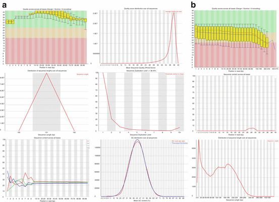
Fig. 6.3

Quality control of raw sequencing reads. (a) Outputs from the FastQC software showing, from top left to bottom right; quality value distribution per position; distribution of mean quality values per reads; reads length; duplicates level; base composition; GC content. (b) Examples of bad-quality profiles from top to bottom; low-quality values per base; fraction of N bases; reads length distribution with very small sequences

6.2.2.4 Reads Alignment on a Reference Genome

The reads alignment (also called reads mapping) is the process of figuring out where in the genome a sequence is from. The reads alignment differs from the reads de novo assembly in the way that it is based on a known reference genome. De novo assembly strategies are usually used to reconstruct DNA contigs or RNA transcripts without reference genome. Note that some strategies have been developed using both reads mapping and reads assembly to reconstruct highly rearranged tumor genomes. In terms of complexity and time requirements, de novo assemblies are orders of magnitude slower and more memory intensive than reads alignment (Fig. 6.4).

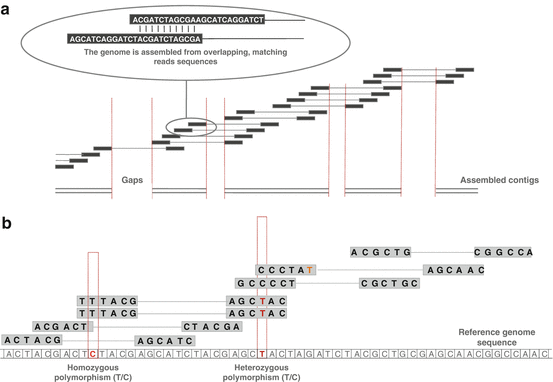
Fig. 6.4

Difference between genome assembly and reads alignment. (a) Reads are aligned and merged together in order to reconstruct the original sequence, usually represented as contigs. (b) Reads alignment on a reference genome. Misalignments can either represent a true variant information or a sequencing error

Reads alignment can be seen as an (in)exact matching problem, i.e., given a long text and a much smaller pattern, the goal is to find the location in the text where the pattern occurs (allowing a predetermined number of misalignment).

Two main challenges have to be faced up. The first one is practical: if the reference genome is very large (3.10⁹ nucleotides for the human genome) and if we have hundred of millions of reads, how quickly and efficiently is aligning these reads on the genome? The second is methodologic: sequencing errors or polymorphisms as well as reads coming from repetitive elements make the problem much more difficult in practice. In some cases, detecting the unique position on the genome where the read belongs to is impossible. If so, the program should choose to report multiple possible locations or to select one location randomly.

Understanding in details the algorithm of an alignment software is usually not necessary to use it in practice. In the following section, we will focus on the practical matters and the rationales of reads alignment.

Compression and Indexes

The first step of the reads alignment is the choice of the reference genome to work with. The reference genome has to be indexed before running the alignment. Like the index of a book, the index of the reference genome allows the program to rapidly find shorter sequences embedded within it. Several strategies have been proposed to build indexes based on a data structure allowing an efficient memory storage and a rapid course of the data. The Burrows-Wheeler transform (BWT) is a compression process that reorders the genome in a way that exact repeated sequences are collapsed together in the data structure (Fig. 6.5). It is reversible, so that the original sequence can easily be reconstructed from the transform. The transformation was originally discovered by David Wheeler in 1983 and was published by Michael Burrows and David Wheeler in 1994. This method is used by popular reads alignment software, such as Bowtie (Langmead et al. 2009), Bowtie2 (Langmead and Salzberg 2012), GEM (Marco-Sola et al. 2012), and BWA (Li et al. 2009). These softwares are fast allowing the alignment of 100 millions reads in a few hours, requiring a few gigabytes of memory. The main limitation of this approach is the number of mismatches or gaps allowed in the read. However, as sequencing becomes increasingly accurate, this limitation is likely to become less important for species with relatively low polymorphism rates.

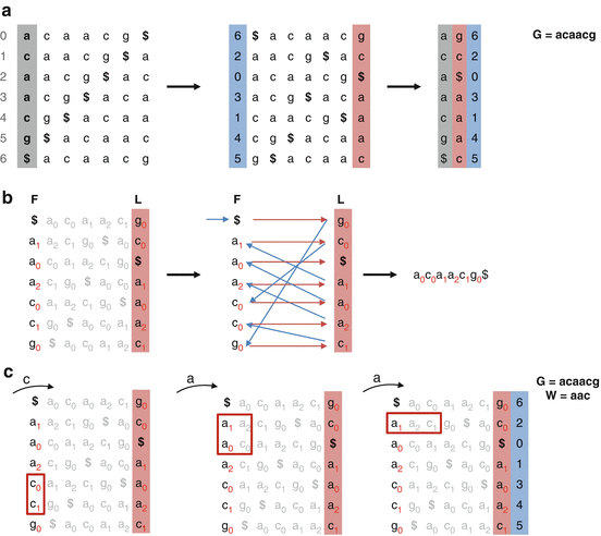
Fig. 6.5

Burrows-Wheeler transform and exact mapping. (a). Burrows-Wheeler transform (BWT). The BWT transformation can be achieved in three steps. First, we apply a rotation on the string G by repeatedly taking a character from one end and sticking it on the other. The rows are then sorted by alphabetical order. The final column represents the BWT transformation. (b) LF mapping. The BWT is reversible through LF mapping which is based on the property that the ith occurrence of a character c in the last column has the same rank as the ith occurrence of c in the first column. (c) Exact matching. The BWT can be used as an efficient index of G (FM-index). The matching starts by finding the rows beginning with the shortest proper suffix of W. Then, because only the F, L, and rank columns are stored in the index, the LF mapping strategy is used to extend the suffix until exact matching

Searching

Without considering the sequencing errors, the existing polymorphisms between the reference genome and the real sequence usually require more flexible strategies allowing mismatches and gaps. In the context of oncology and DNA sequencing, allowing gaps is mandatory to detect variants and insertion/deletion events. BWT is extremely fast for finding exact alignments, whereas dynamic programming is flexible and allows gaps detection. In this way, an alignment is usually characterized by a score that reflects the global match, mismatch, and gap rates. The higher is the score, the better is the alignment. The scoring system can also used the raw Phred quality of each nucleotide. It is thus more likely to observe a true mismatch at a low Phred quality position (Fig. 6.6). Changing the scoring system of the software will change the number and quality of reads that map to the reference and the time it takes to complete the alignment. It is also important to notice that many alignment softwares are based on heuristics. This means that the reported alignment is not guaranteed to be the best one. The alignment accuracy can usually be defined but at a cost of intensive computing time.

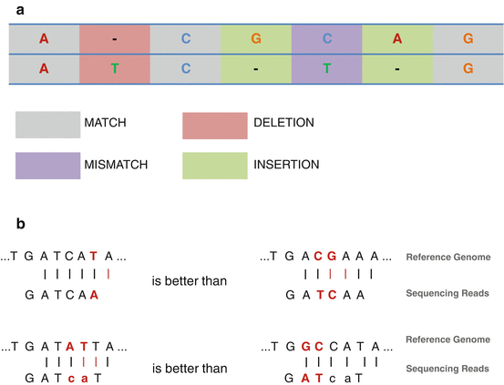
Fig. 6.6

Rationale of reads alignment. (a) Definition of match, mismatch, insertion, and deletion. (b) The goal of reads alignment is to find the best reads position in a reference sequence. In this way, allowing one mismatch is better than allowing two mismatches. In addition, reads mapper is usually able to use base quality values. Therefore, allowing two mismatches on low quality bases (lower case) is better than mismatches on high confidence bases

Since sequencing technologies are now able to generate longer reads, recent alignment softwares now propose both local and global alignment strategies. Global alignment is appropriate for sequences that are expected to share similarity over their whole length, meaning that the entire read must be aligned on the reference genome, whereas local alignment is appropriate when the sequences may show isolated regions of similarity, meaning that only a subpart of the read can be aligned on the reference. The unmapped part is usually returned as soft-clipped sequence occurring at one or both ends of the read (Fig. 6.7).

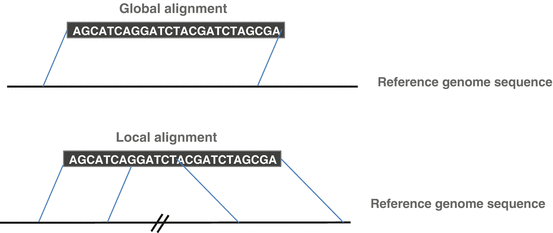
Fig. 6.7

Global versus local mapping strategy. Global (or end-to-end) strategy will align the entire read sequence on the reference genome. Local alignments find the best alignments of sequence segments, which can be separated and in any order

Reporting

Understanding how alignment positions are reported by the software is extremely important for downstream analyses. Depending of the genome complexity and size, a large majority of reads is expected to be uniquely aligned on the reference genome. Keeping only those unique reads ensures a high-quality alignment but excludes from the analysis all the repeated regions. According to the biological context, reads aligning to multiple positions can also be informative. This is, for instance, the case of reads spanning genes and their pseudogenes or reads aligned to intronic repetitive sequences.

Paired-end sequencing comes with a prior expectation about the relative orientation of the mates and the distance separating them on the original DNA fragment. In most of the case, both mates are first independently aligned on the reference genome. An additional step is thus required to pair both alignments trying to promote concordant reads pairs. A concordant read pair is defined by an expected distance between the two mates and a concordant mate orientation. Some aligner such as BWA should be able to promote a suboptimal position if its mate is hanging around. This is useful to anchor reads in repeats.

Once the alignment is performed, the mapping quality score (MAQ) of a given read quantifies the probability that its position on the genome is correct. The mapping quality is encoded in the Phred scale (see 1.) where P is the probability that the alignment is not correct.

The probability is calculated as:

P = 10 ^(−MAQ/10)Where MAQ is the mapping quality. For example, a mapping quality of 40 = 10 to the power of −4, meaning that there is a 0.01 % chance that the read was aligned incorrectly.

Only gold members can continue reading. Log In or Register to continue