Fig. 11.1
An example of regular breathing
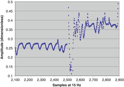
Fig. 11.2
An example of highly irregular breathing
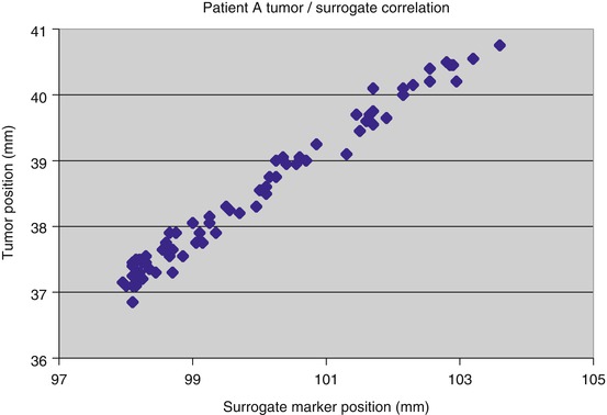
Fig. 11.3
A sequence of measurements of tumor position and chest marker position, showing a tight correlation over time [35]
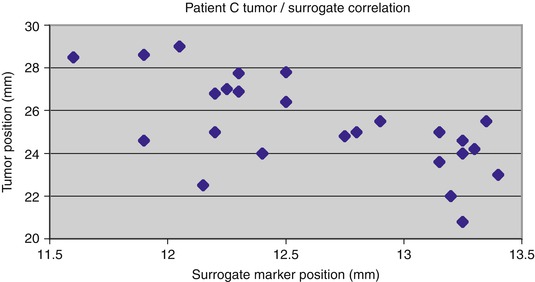
Fig. 11.4
An example of tumor and chest marker positions that do not maintain a tight correlation over time [35]
These characteristics of breathing and tumor movement make it exceedingly difficult to devise a mechanical model of breathing that can accurately and continuously describe the movement of the anatomy and enable its prediction. The problem is instead a good candidate for a machine learning approach, using general algorithms that can learn to imitate the movement patterns via training on examples of the patient’s actual breathing. The algorithms must furthermore be capable of continual adaptation to changes in the motion patterns, through methods of continuous retraining as the patient breathes. Many different prediction algorithms have been investigated (see, e.g., [6]). Among them, adaptive neural networks have been found to be an effective machine learning approach to this problem. They are the focus of this chapter.
11.2 Using an Artificial Neural Network (ANN) to Model and Predict Breathing Motion
The basic mechanism for maintaining beam alignment with a moving tumor is illustrated schematically in Figs. 11.5 and 11.6. Figure 11.5 is an “open loop” control architecture that is appropriate for either a gating or a beam tracking scheme. The tumor moves solely under the influence of patient movement (e.g., breathing). Respiration and/or tumor position sensors provide the input to the loop. The corrective signal propagates through various system components, each of which takes some time to react, resulting in a cumulative delay before the beam responds with the correction. Figure 11.6 is a “closed-loop” architecture in which the system’s response combines with the patient’s anatomical movement to influence the position of the target relative to the beam isocenter and thus the input to the loop. This is required for an adaptive system that moves the couch and patient relative to the beam as the tumor moves, so as to keep the tumor at a fixed position (set point) in space. In this case, respiration and couch shifts combine to move the tumor. In both architectures, the tumor position can be established either by following a surrogate breathing signal that correlates with tumor motion or by directly observing the tumor’s position or both.
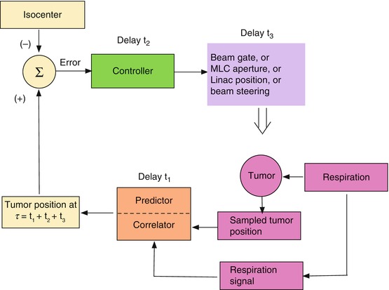
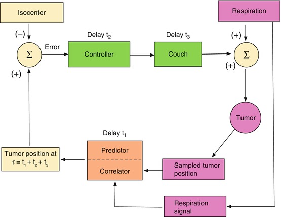
Fig. 11.5
An open control loop architecture for maintaining beam and tumor alignment
Fig. 11.6
A closed-loop beam alignment architecture
The subject of this chapter is the control loop element identified in Figs. 11.5 and 11.6 as the “correlator/predictor”. This element receives as input some measurement of breathing and provides the anticipated position of the tumor as input to the beam or couch controller. To allow for control loop delays, the “correlator/predictor” must emulate the patient’s breathing in order to predict the future respiratory signal and/or tumor position.
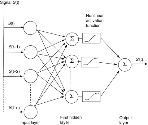
An artificial neural network (ANN) is a trainable machine learning algorithm. One form that is very useful for predicting a signal amplitude has the basic architecture shown in Fig. 11.7. In this kind of application, we have some measured signal S(t) as input and a future instance of that signal S(t + n) as the output target. The job of the ANN is to make an estimate S’(t + n) of the future target signal from samples of the input signal. The input layer of the network is provided with discrete measurement samples from the past signal history, the hidden layers compute weighted combinations of the input data, and the output layer delivers an estimate of the target signal at a future time. In Fig. 11.7 the target signal is a future sample of the input signal, in which case the network is trained to imitate the input signal so that it can predict its future behavior. When the target signal finally arrives at time t + n, the prediction S’(t + n) is compared to it, an error is computed, and this error is used to adjust the network weights so as to produce a more accurate prediction of the next sample. Figure 11.8 shows a configuration to use the input signal S(t) to predict a different signal P(t) that is correlated in some way with the input signal. In this case the network is trained to predict the correlated target signal from the input. The target prediction might be for the present moment or some future time.
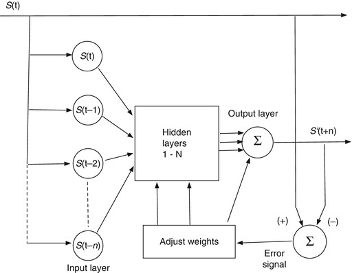
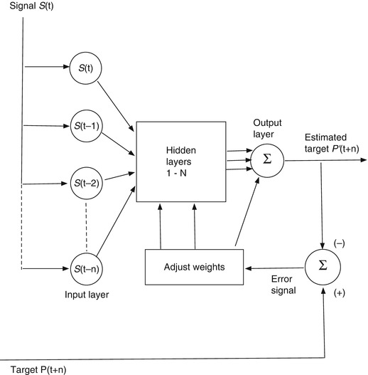
Fig. 11.7
An artificial neural network architecture to predict a signal amplitude S(t)
Fig. 11.8
An ANN configured to predict a different signal P(t + n) that is correlated with the input S(t)
In our breathing prediction problem, we identify the input data with a sequence of discrete measurements of the patient’s breathing. This could be as simple as the time history of the amplitude of a single breathing signal, such as a moving marker [29] or spirometer signal [15, 54], or it could comprise simultaneous measurements of multiple breathing signals [53]. If we are only interested in predicting breathing movement to compensate for a treatment system’s lag time, then the target signal would be a future instance of the patient’s measured breathing, and the network’s output would be an estimate of that future instance. If we are interested in deducing the tumor position from the measured breathing signal, then the input signal would be a breathing surrogate measurement, and the target data would be a measurement of the tumor’s spatial position at some particular time. It could be the tumor position at the present time, in which case the ANN makes a spatial correlation between the tumor and breathing motions, or it could be the future position of the tumor, in which case the network performs both a correlation and a temporal prediction to arrive at a good estimate of the tumor location.
11.3 Neural Network Architectures for Correlation and Prediction
11.3.1 The Single Neuron, or Linear Filter
We can introduce the basic computational components of an artificial neural network for correlation and prediction by considering a simple network configured to predict the future amplitude of a single breathing signal sampled at discrete time intervals. It begins with a single neuron, as shown in Fig. 11.9 (This has historically been known as a linear perceptron). The input is the amplitude history of the measured signal S(t), sampled at n intervals of τ seconds. For breathing, which has a period of a few seconds for most people, τ might be on the order of 100 ms. We take the N most recent samples. Each sample is multiplied by a weight w i and the N samples are summed:
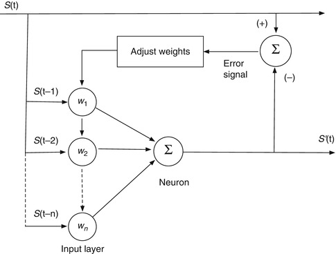
If we stop here, we have a simple linear filter, where S’(t) is the filter’s estimate of the signal amplitude at the present time, based on the previous N samples. S’(t) is compared to S(t) and the error is used to adjust the weights until the difference is minimized. If we want it to predict S at some future time t + Δt, rather than the present, we wait Δt seconds for the actual signal to arrive, compare it to S’ to find the error, and adjust the weights accordingly.
Fig. 11.9
A simple linear filter for prediction
(11.1)
The linear filter (i.e., a single neuron) in Fig. 11.9 and Eq. 11.1 can do a reasonable job of predicting breathing, provided that the pattern isn’t too changeable or irregular [31]. It provides a starting point to introduce several basic elements in the development of ANNs for prediction and correlation.
The weights are initially optimized in the training stage. For a basic signal prediction filter, this typically consists of presenting the filter with prerecorded signal histories that are representative of the signal that one ultimately wants to predict. For example, if one wants a filter customized to emulate and predict a particular patient’s breathing, one begins by recording a segment of the patient’s breathing signal. This is presented to the filter incrementally via a sliding window that is N samples wide. The filter gets a set of N samples up to a time t at the inputs, makes a prediction for t + Δt, compares the prediction to its target (which is the recorded signal at t + Δt), adjusts the weights, steps forward one sample, and repeats the process. This is an example of supervised sequential training. Sequential training has the advantage that, as the filter is presented with new breathing data that it hasn’t seen before, it can continue the process, retraining continuously to adapt to new breathing patterns.
The initial training process must be done in such a way that it doesn’t “see” future samples in the training stage before they would actually arrive in real time.
The simplest training algorithm for a linear neuron is the LMS (least mean square) method. Let S i be the vector of N input samples from the ith training signal history, let W i be the vector of N weights assigned to the inputs, and let ε i be the difference between the predicted and target signal sample. The updated weight vector is
where α is a parameter that determines the speed of convergence. In the case of sequential training, each training signal history S i is simply the previous signal history advanced by one sample.
(11.2)
11.3.2 The Basic Feedforward Artificial Neural Network for Prediction
Soon after the single-neuron perceptron was proposed as a primitive machine learning algorithm for pattern recognition, Minsky proved that it, and any linear combination of neurons performing the function of Eq. 11.1, could only do linear discrimination and was incapable of performing even a simple exclusive-or function [28]. This led to the development of nonlinear networks of neurons for more complex pattern recognition and signal processing. Figure 11.10 is a schematic of the simplest nonlinear neural network – a feedforward network with one hidden layer – for signal prediction. The inputs are distributed in parallel to two or more neurons like the one in Fig. 11.9 (the simple linear filter). These make up the “hidden” layer. (The layer is “hidden” because it can’t be reached directly from the outside.) The output x of each neuron is passed through a nonlinear “activation” function f(x) (the sigmoid function in Eq. 11.3 is the most commonly used), weighted, and summed with the others in the output neuron, which delivers the final signal estimate.
The activation function must be nonlinear; otherwise, the network is reducible to a single linear neuron and nothing is gained.
Fig. 11.10
A basic feedforward network with one hidden layer of neurons and a single neuron in the output layer
(11.3)
(11.4)
11.3.3 Training the Feedforward Network
Each input to each neuron in the hidden and output layers in Fig. 11.10 has an independently variable weight. However, the weights in the hidden layer are “blocked” from the output signal error by the nonlinear activation function. This prevents a simple linear generalization of the LMS algorithm in Eq. 11.2. The problem is solved by the method of error back propagation.
Although the basics of back propagation can be found in any textbook on neural networks (e.g., [12]), there is some advantage to providing them here, using the simple two-layer network in Fig. 11.10 as the architecture. Let layer 1 be the hidden layer and layer 2 be the output layer (in this case just one neuron). Let the index i apply to the data samples and j to the number of neurons in layer 1 (and also the equal number of input weights to layer 2). Let W 1, j be the vector of weights for the jth neuron in layer 1 (with components w 1, ji ) and W 2 be the weight vector for the output (layer 2) neuron (with components w 2, j ). The outputs of the layer 1 neurons are x 1, j before activation and y 1, j after activation. The error in the predicted output signal is ε.
In the forward pass, the delta is calculated for layer 2:
 In the backward pass, the deltas for layer 1 propagate through the derivative of the transfer function:
![$$ {D}_{1,\ j}=\left[{y}_{1,\ j}\left(1-{y}_{1,\ j}\right)\right]\left[{D}_2{w}_{2,\ j}\right]. $$](/wp-content/uploads/2016/10/A320877_1_En_11_Chapter_Equb.gif) The incremental changes to the weights in the two layers are then calculated (in this example via LMS):
The incremental changes to the weights in the two layers are then calculated (in this example via LMS):
In addition to LMS, there are a number of other algorithms that can be used to update the weights [12, 13]. Regardless of which one is used, there are some general principles to be followed to get the best results. The first step is to initialize all of the weights. The usual practice is to choose them randomly, because this gets the neurons acting independently. However, there is always some chance that a random initialization will come up with an unfavorable filter that performs badly. This can be avoided by performing the random initialization and subsequent training multiple times while testing each fully-trained filter on an independent validation signal. The set of weights that does the best job of predicting the validation signal becomes the optimal filter for application to test signals. The validation signal can be any part of the prerecorded signal that wasn’t used for training.
It is also generally the case that a single pass through the training data will not result in optimal convergence of the weights. It is therefore customary to run through the training data repeatedly, starting each subsequent training pass at the weights from the prior training pass. Each pass is called an epoch. However, there is the risk of overtraining the filter after too many epochs. In this case the filter becomes completely optimized to emulate the training data but cannot generalize effectively to signals it has not yet seen. This can be avoided by testing each epoch of trained filter on the validation data and terminating the training when the filter’s performance on the validation set is clearly worse than its performance on the training data.
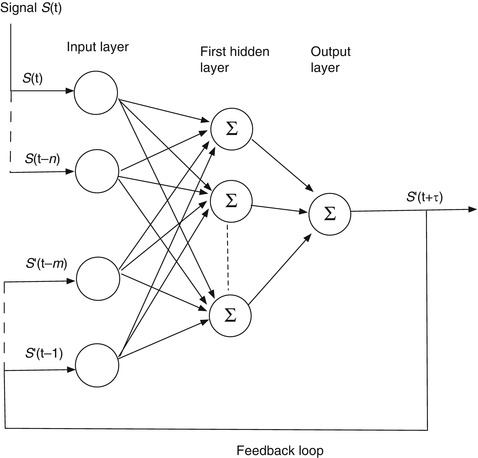
11.3.4 The Recurrent Network
A recurrent network is a closed-loop feedback architecture in which signals from the hidden and output layers are fed back to previous hidden layers and/or to the input layer. This architecture is inspired by the observation that the human brain is a recurrent network of neurons. In Fig. 11.11, a simple recurrent network for prediction feeds the previous m − 1 predictions back to the input layer at each time step S(t) of the input signal. The output signals are held back by the prediction interval τ before they are supplied to the input, so that the error between S(t) and S’(t) can be computed and used to update the weights. The hoped-for advantage is that the raw input data from the (potentially noisy) measurements is supplemented by filtered data from the outputs that will smooth out the network’s response. A recurrent network can be trained in the same way as a feedforward network, e.g., via back propagation.