Application of Machine Learning for Multicenter Learning

Fig. 6.1

Visual representation of the sample ontology

Table 6.1

RDF representation of a patient based on the ontology of Fig. 6.1

Subject	Predicate	Object
mySet:patient1001	rdf:type	ncit:C16960
mySet:patient1001	myOntology:hasFirstName	“John”^xsd:string
mySet:patient1001	myOntology:hasLastName	“Doe”^xsd:string
mySet:patient1001	myOntology:hasBiologicalSex	ncit:C20197
mySet:patient1001	myOntology:hasAge	67^^xsd:integer

Unique Resource Identifiers and Linked Data

To assure semantic interoperability, we will use the concept of unique resource identifiers (URIs), which is incorporated in the RDF specification. The RDF specification states that all resources (concepts and predicates) need to have a URI, which can be a unique resource locator (URL; e.g., http://www.mydomain.org/ontology#hasFirstName) or a unique resource name (URN; e.g., myOntology:hasFirstName). This means that someone needs to own a domain name (e.g., mydomain.org) and is administrator of this domain. If this is the case, he or she can make unique URLs for this domain, for example, to create a unique URI for patient 1001 (e.g., http://www.mydomain.org/rdf#patient1001). If the domain administrator assigns a specific sub-path of the domain to a dataset (called a namespace), for example, http://www.mydomain.org/rdf#, then this sub-path can also be substituted by a prefix, for example, “mySet”. This namespace can then be used to shorten the notation of a unique patient, as shown in Table 6.1. This concept of unique resources also holds for ontologies, where in Table 6.1 the prefix “myOntology” can be used to define the namespace http://www.mydomain.org/ontology# and the prefix “ncit” refers to the unique location of the NCI thesaurus. As everyone should use the same, unique namespaces, the use of URIs enforces semantic interoperability. Therefore, semantic interoperability is enforced within the Resource Description Framework.

Next to the enforcement of semantic interoperability, the use of URIs has a second benefit, namely, the possibility of linked data. As every resource has its unique URI, an RDF store at site A may point to a resource at site B by using the URI of the resource at point B [4]. For example, if a patient underwent a diagnostic scan at hospital A and was treated in clinic B, then clinic B can specify the treatment and link it to the patient resource with the unique URI used in hospital A.

Querying Using SPARQL

We have described how data can be represented in RDF, and how URIs enforce semantic interoperability and linked data. But how can we retrieve this data from an RDF store? To query these RDF stores, the W3C has adopted the SPARQL protocol and RDF query language (SPARQL) [24]. Most RDF stores have integrated a SPARQL endpoint in their RDF store. A SPARQL endpoint is the public interface to receive SPARQL queries and return a result table, all using the HTTP protocol. In contrast to SQL queries, SPARQL queries do not search tables due to the underlying RDF store structure. SPARQL queries perform pattern matching on the triples in the triple store, where variables can be used to retrieve unknown values or to dynamically link values. For example, the query in Listing 6.1 will try to retrieve the first name, last name, and age for all patients. We will shortly describe the lines in this query example.

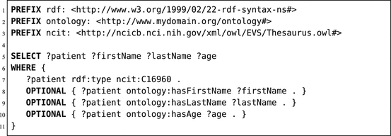
Listing 6.1

Basic SPARQL query retrieving patient resources, related first and last names, and age of patient data stored in an RDF store, based on the ontology defined in Fig. 6.1

On line 1–3, the shorthand (prefix) notations for URL locations are defined. Line 5 defines the variables retrieved from the pattern matching; these variables have to start with a question mark. Lines 6–11 define the actual pattern searched for. As shown in Listing 6.1, our basic pattern is to retrieve all patient resources which have a predicate called “rdf:type,” which refers to the terminological code of a patient, defined in the NCI Thesaurus (using the prefix “ncit:,” which is replaced by the full URL at line 3). Afterwards, we extend our pattern match by including extra properties for every resource linked to the patient resource. If the linked resources of the patient variable have a predicate matching to our specified property (in our ontology), then the variable firstName, lastName, or age will be filled with the found value. If not found, then the query will return the patient resource URI; however, the variables firstName, lastName, or age are not filled in (due to the “OPTIONAL” keyword).

Next to querying one RDF store, a SPARQL query can also be federated to multiple stores. This is an advantage in regard to multicenter learning, as a single query can retrieve data from multiple sources. Due to the structure of RDF stores, data residing in geographically separated RDF stores can easily be merged, as the data structure is the same for all stores (1 table; 3 columns) and all RDF stores should use URIs. Federation can be done both horizontally (different patients in different RDF stores) or vertically (information of a single patient stored in multiple RDF stores). An application of horizontal federation in SPARQL queries is shown in Listing 6.2; an application of vertical federation is shown in Listing 6.3. In these examples, we will use the “SERVICE” command of SPARQL to identify the execution of a subquery (or pattern match) on a different SPARQL endpoint. In Listing 6.3, we used the exact same pattern query in both services/subqueries (line 7–19). Both subqueries are sent to the respective endpoints, and the subquery results are merged at the federation endpoint. Finally, the requested variables are returned to the requesting application or user. In Listing 6.3, both services have different patterns to match. The first service (line 7–11) searches for all patients and their first/last name on SPARQL endpoint 1. The second service (line 13–15) will reuse the patient resources found in endpoint 1 and tries to find patterns matching the hasAge predicate for these given patient resources. When found, it will use the object linked to the hasAge predicate (in this case a literal of type integer) and store it in the variable “?age”. Finally, the query engine will return the output as one table (using the variables of line 5 as columns), including information retrieved from both endpoints.

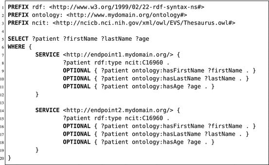
Listing 6.2

An example of horizontal federation in a SPARQL query

Listing 6.3

An example of vertical federation in a SPARQL query

In this paragraph, we have presented an alternative to the widely known relational databases to represent and retrieve data. The use of Semantic Web technology, and especially RDF, has several advantages over relational databases. Especially the meta-structure of RDF (independent of the modeled domain) and the use of URIs are useful with regard to a flexible storage solution while inherently adopting semantic interoperability and linked data.

On the other hand, using Semantic Web technology has some downsides when used in multicenter machine learning. The main downside is that local institute staff needs to be introduced to Semantic Web technologies, in order to maintain these data repositories and endpoints. Furthermore, development in the field of RDF stores/repositories is an ongoing process and is not yet comparable to relational databases in terms of reliability and performance, especially in daily clinical practice. On the contrary, for research projects (where uptime is less critical), the Semantic Web is more favorable because of its flexibility in storage and data structures.

6.2.3 Network Infrastructure

Up until now, we only described how to extract information from multiple sources (databases, image archives) and to apply standardized terminological systems on the data extracted from these sources. Furthermore, we have described how to represent data using the relational database and semantic web technology. In this paragraph, we will combine the topics of the previous paragraphs (Sects. 6.2.1 and 6.2.2) and explain how we can use them together. First, we will describe the institutional infrastructure, after which we will describe the multicenter infrastructure.

6.2.3.1 Institutional Infrastructure

In this paragraph, we will describe several approaches to represent a single point of access for the outside world (e.g., participating sites in the multicenter machine learning setting). We will discuss five different approaches, namely:

Traditional ETL and DWH
Traditional ETL and DWH with an RDF store
Traditional ETL and DWH with a virtual RDF store
Virtual RDF store per institute
Virtual RDF store per source and institute

Traditional ETL and DWH

In the approach using relational databases (Sect. 6.2.2.1), records from different source systems (e.g., EMR, PACS, TPS, and R&V) are merged using an ETL tool (Sect. 6.2.1.1) and converted into the requested data formats following standards used by all collaborating sites (Fig. 6.2). The merged and transformed data are being saved in the DWH database. This database will afterwards be queried when requesting data for machine learning purposes. Therefore, this database needs to be compliant to the ontological structure (among all participating centers). When the ontology is altered, all participating centers need to update the DWH database structure, as well as the transform and/or storage scripts in the ETL tooling.

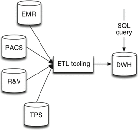
Fig. 6.2

Infrastructure of the traditional ETL and DWH approach

Traditional ETL and DWH with an RDF Store

This approach uses an RDF store on top of the traditional ETL and DWH approach (Fig. 6.3). It enables the possibility to create an institutional DWH instead of a DWH dedicated for the study. Afterwards, the “Database to RDF” conversion application reads the DWH database and transforms the data it into triples, taking into account a given ontology. This RDF store will afterwards be queried when requesting data for machine learning purposes. Only the “Database to RDF” application needs to follow the rules and data structure defined in the ontology. When the ontology is altered (e.g., adding an extra data element), only this database-to-RDF application needs to be altered (when the information is already available in the DWH). Updating the RDF store is done by clearing and repopulation and is performed at specific time intervals.

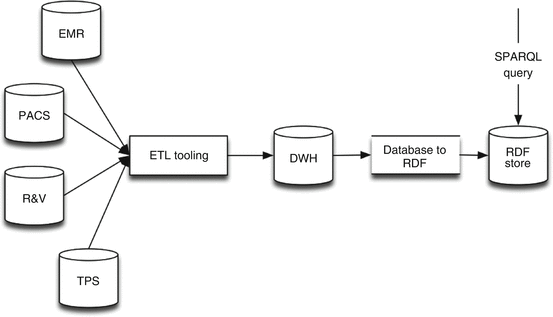
Fig. 6.3

Infrastructure of the approach using a traditional ETL and DWH with an RDF store

Traditional ETL and DWH with a Virtual RDF Store

This approach uses only the database-to-RDF conversion application on top of the traditional ETL and DWH approach (Fig. 6.4). This approach is almost equal to the physical RDF store approach (Fig. 6.3); however, it has one difference in converting data from relational databases to RDF.

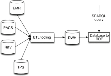
Fig. 6.4

Infrastructure of the approach using a traditional ETL and DWH with a virtual RDF store

In this case, the “Database to RDF” application acts as a SPARQL endpoint, accepting SPARQL queries and returning the result of these queries. There is no data stored, as there is no RDF store, only a SPARQL endpoint. When performing a SPARQL query, the database-to-RDF application will transform SPARQL queries into SQL queries and executes these SQL queries on the DWH. In regard to maintenance, this option holds the same requirements as using the physical RDF store. The only difference is the absence of an intermediate RDF store, resulting in real-time results of the data available in the DWH.

Virtual RDF Store per Institute

As the DWH usually is not a real-time representation of the clinically available data, this approach removes the DWH and directly queries the source systems. In this approach, the database-to-RDF application is functioning as a SPARQL endpoint without an RDF store and converts SPARQL queries into SQL queries for the different source systems (Fig. 6.5). It therefore creates challenges for the database-to-RDF application, as it needs to transformation data (to convert local terms to standardized terms), which was previously done by the ETL tooling. If multiple source systems are involved, the database-to-RDF application merges the results from all sources and presents them as a SPARQL query result. The main benefit of this approach is that we can query for real-time data, rather than have to wait before the data is added to the DWH. Furthermore, data redundancy of the intermediate storage (the DWH) is not needed, reducing the need for storage resources. However, the main disadvantage is with regard to performance, as data and queries are transformed on the fly.

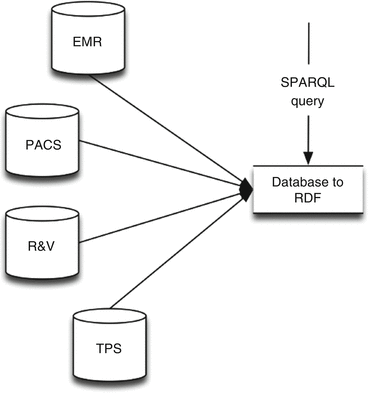
Fig. 6.5

Infrastructure using only a virtual RDF store

Virtual RDF Store per Source and Institute

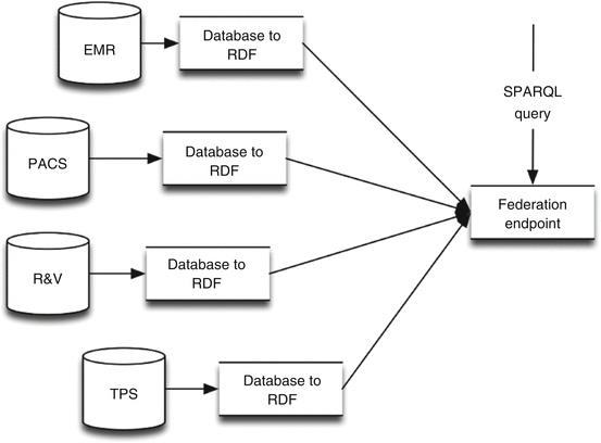
This approach is almost similar to the “Virtual RDF store per institute” approach, however, with differences in data transformation and federation (Fig. 6.6). First, every local data source will get a SPARQL endpoint, using, for example, the database-to-RDF application. This application will convert the data from the source system into RDF, compliant with the ontology used in the multicenter setting. Afterwards, the central federation endpoint will be used to merge all triples from all database-to-RDF applications/sources (vertical federation). In this setting, one SPARQL query will be sent to the federation endpoint. This federation endpoint will split the SPARQL query into several sub-SPARQL queries and execute these SPARQL queries on the SPARQL endpoints placed on top of the data sources. Afterwards, the federation endpoint will merge the results and return the merged result set to the application/user performing the query. The benefit of this approach is the distribution of computational resources to reduce the query execution time. The drawback is that $$ n+1 $$

applications (where n is the number of database-to-RDF applications) are need to be maintained and updated when the ontology changes.

Fig. 6.6

Infrastructure using a virtual RDF store per source and institute

6.2.3.2 Multicenter Infrastructure

In the previous paragraph (Sect. 6.2.3.1), we described the institutional infrastructure options to create one façade or data query endpoint for every center. It depends on whether we are using centralized or distributed machine learning (Sect. 6.3) and whether we need an additional computation unit (e.g., a dedicated or virtual server) in each center. Both distributed and centralized approaches can be implemented using relational databases or Semantic Web technology; however, the decision regarding data representation techniques needs to be made upfront and accepted by all participating centers. In this paragraph, we will first describe the centralized machine learning infrastructure and afterwards move towards the distributed infrastructure.

Centralized Multicenter Infrastructure

The general overview for the centralized multicenter infrastructure is shown in Fig. 6.7. The participating sites are displayed as a data store, as we do not need to know what the institutional infrastructure looks like. This approach gives participating centers the opportunity to establish the institutional infrastructure according to local policies. Additional to all institutional entry points, a central machine learning server (performing the computations) and a central federation point need to be set up. The central federation point will perform the horizontal federation between participating centers. To ensure privacy (Sect. 6.2.4), the data stores of the participating centers may limit external access by only allowing access from the central federation point. The central machine learning server will accept and execute algorithms (including queries to execute on the central federation point). After the algorithm has finished, it will return the outcome of the computation to the external source which sent the job (algorithm + query).

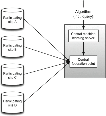
Fig. 6.7

Centralized multicenter infrastructure

Distributed Multicenter Infrastructure

The distributed multicenter infrastructure is different from the centralized version with respect to computational locations. As shown in Fig. 6.8, the central federation point has been removed, and local computation units (machine learning slaves/agents) have been introduced. In this infrastructural setting, the central machine learning server (master server) is a coordinating server. When a job (algorithm + query) is submitted to the central ML master, the algorithm is being split into smaller sub-algorithms. These sub-algorithms and queries are packed into sub-jobs and sent towards the local computation units. They will query the local endpoint and execute the sub-algorithm. After finishing the sub-algorithm, the results are sent back to the central ML master, which gathers the results from all local endpoints. The central master will then determine whether it will perform a new sub-job on all endpoints or aggregate values and sends the final (aggregated) result back to the job-submitter. More information regarding the actual execution of the algorithm in a distributed setting can be found in Sect. 6.3.2.

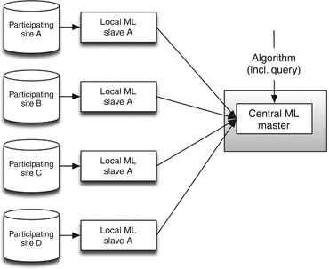
Fig. 6.8

Distributed multicenter infrastructure

6.2.4 Privacy Preservation

For both distributed and centralized multicenter infrastructures, privacy preservation is a major topic to take into account. If correctly implemented, the distributed multicenter infrastructure is generally more secure as the results of the algorithm (e.g., a predictive model) are transferred instead of the source data. However, this does not mean that the issues concerning privacy preservation are solved. For example, it is still possible to retrieve metadata about a dataset of one patient. In this section, we will address several options for privacy preservation, ranging from pseudonymization to irreversibly modifying the original datasets. Despite of all the options described below, we have to state that, in our opinion, there is no standard method to ensure privacy preservation. The researcher/designer of the infrastructure will always have to find a balance between the loss of information and the anonymity of participating patients.

Pseudonymization

The first option for privacy preservation is bidirectional pseudonymization of patient identifiers, for example, replacing patient names and hospital’s patient identification numbers by study-specific alternatives. This can be achieved by maintaining a two-column table, where one column contains the patients identification number and the second column contains the study identification number for this patient. Variations to this concept may apply, for example, using an extra column to maintain the study where this mapping applies to. Typically, the pseudonymization of hospital to study identification numbers is done during the transform part of the ETL process. Other patient identifying information (e.g., first and last names) can be replaced by the same study ID or may not be incorporated and thus removed during the ETL process.

The second option is to use an unidirectional pseudonymization algorithm, for example, by hashing patient identifiers (e.g., using an SHA-{1–3} algorithm). This hash should be unidirectional, meaning that the pseudonymized patient identifiers cannot be reversed to the original identifiers. Unidirectional pseudonymization might be more appropriate than bidirectional pseudonymization, however might introduce problems when study data are needed to be linked to the actual patients. For example, when study results show a worse outcome for specific patients and when it is immoral to withhold this information to these patients.

Data Obfuscation

When using strict inclusion criteria with rare variables, it might be that the resulting dataset is very small and patients might become identifiable by combination. For example, if only two patients match some inclusion criteria and the biological sex (which is a requested variable) is different in both patients, we can identify these patients when querying local source systems. This issue holds for both the centralized and distributed multicenter infrastructures. To reduce the chance of compromising the anonymity of patients, Murphy and Chueh [21] introduced a method for data obfuscation where (especially in the case of a small number of events/patients) results are obfuscated by returning a random value within a specific range based on the actual value. This method does not circumvent the problem completely, as someone with bad intentions is able to approximate the original value by sending the same request multiple times. To circumvent these actions, Murphy and Chueh proposed to implement an audit system, where performing the same query multiple times within a specific time span will result in a request denial. In this way, the system returns a value not completely representing the actual value however returns a value within a tolerable margin (when not exceeding the maximum number of requests).

Only gold members can continue reading. Log In or Register to continue