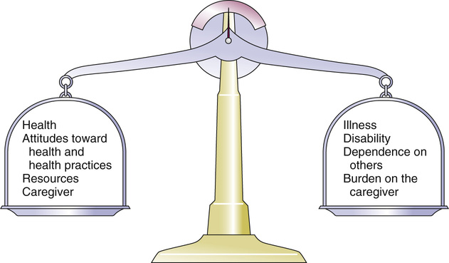
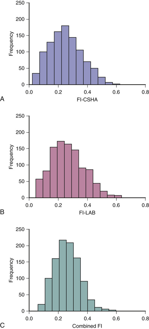
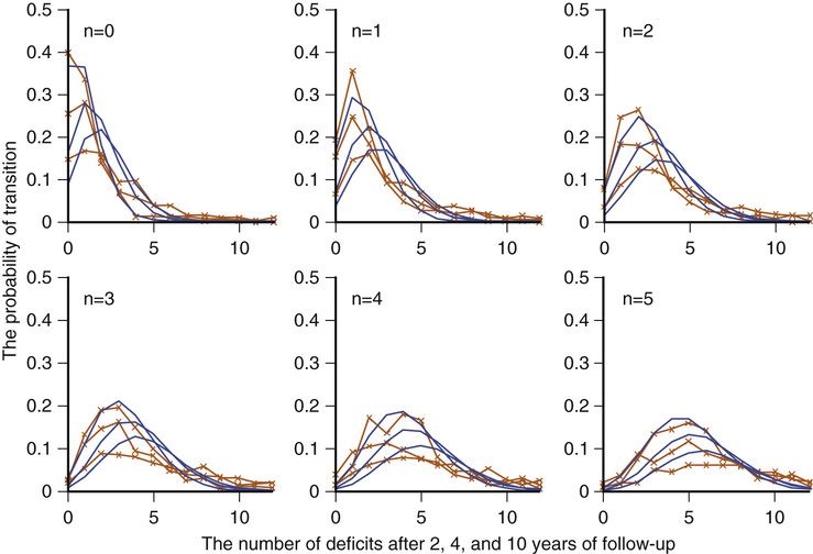
Overview of Complex Networks

The idea of complex networks being susceptible to formal analysis, and of those analyses extending to biologic systems and in particular, medical applications, is proving to be an important conceptual advance.^10,11 Understanding how networks operate from subcellular levels on¹² appears to have transformative potential. In general, a network can be understood as a collection of items (called nodes or vertices) defined by the connectedness of the items (with connections also known as edges). For network purposes, the items are defined by their connections, such as whether they have many or few connections or the distance between one node and the next. As it turns out, a wide array of sets of items shows network properties, from how items in a physiologic system interact to how emails get answered to how scientists cite the work of others. Network properties define types of networks. For example, scale-free networks follow a power law relationship and are marked by many items (nodes), with few connections, and a few with very many connections. Airports are one such example, with a few heavily travelled international hubs, then more regional hubs, and finally a large number of local airports that might only have a few flights a day.

In contrast to heterogeneity in the distribution of connections between nodes found in a scale- free network, small world networks have a more homogenous distribution. Small world networks have many nodes that are highly connected, with short path lengths. Small world networks have been analyzed in relation to Alzheimer disease to show that it is characterized by widespread loss of connectivity, reflected in increased path lengths between functional brain areas.^13,14 Network analyses are relatively new, so that the area remains somewhat tricky. The several challenges are both in our understanding of how network connectivity arises and in technical matters, such as clustering around electroencephalographic or magnetoencephalographic sensors might give spurious connections between nodes. Advances, however, are being made swiftly, so that understanding Alzheimer disease and other brain illnesses as types of disconnections of usual cortical activity can yield insights into the normal functioning of neural networks and how they become disrupted by disease.

Even recognizing that these are initial steps, progress can be made in relation to aging. Network theories of aging are not new, and many dozens of papers have elaborated them. A few recent papers have incorporated complex network analyses. One network model of aging introduced the interdependence of fault-prone agents on one another.¹⁵ The model showed that aging patterns do not depend on the details of the network structure. This suggests that aging is a widely distributed systemic effect, and its features do not depend on exactly which things go wrong, given the multiplicity of things that subtly go awry.¹⁶ Our group, in a simulation study, found that deficit accumulation is responsible for the observed slowing down in the rate of repair of interconnected nodes. The model reproduced not only the major patterns of deficit accumulation observed in a wide variety of countries, but also the Gompertz law of the exponential increase in the rate of mortality with age.¹⁷

The translation of these ideas into tractable clinical insights remains challenging. It is evident that aging humans constitute aging systems, both as individuals and as groups. Similarly, within the human organism, different organ systems and host environment interactions can be viewed as complex networks.^{11–14,17–20} Even so, the specification of complex networks in relation to organ systems—where does the vascular system end and the immunologic system begin?—often results in some arbitrariness. Such arbitrariness is best not ignored when considering a phenomenon as all-encompassing as the passage of time. Furthermore, how to specify the interconnectedness of organs in the body as people age is not clear. It is clear, however, that there is an interconnectedness of health characteristics (interdependence of variables). For now, we limit ourselves to the observation that network analysis allows a great deal of information about the state of a system (e.g. the degree of interconnectedness) to be summarized as a single number and to come from a set of numbers with characteristic distributions. This is the insight that has motivated our particular approach to understanding aging, and especially frailty, in relation to the extent to which people accumulate health-related deficits. Our claim is that an individual’s state of health can be summarized by a single number—the frailty index—and that the properties or behavior of that number (e.g., how the frailty index changes with age) can be considered as an area of investigation in and of itself. To continue that example, we have shown that the distribution of the frailty index with age has distinctive characteristics.^21,22 These characteristics can be studied using network models, which offer an apparatus for such analyses, based on stochastic dynamics.²³ One example is the idea that heterogeneity (here, of the distribution of the frailty index with age)^21,24 arises as a consequence of the stochastic dynamics of complex systems. This approach to studying heterogeneity can be readily summarized using a network approach and has had wide applicability from cortical networks in Alzheimer disease²⁵ to capital markets²⁶ to gas furnace pressures.²⁷

Frailty in Relation to Deficit Accumulation

The fundamental idea of the frailty index is that the more deficits that people have (the more things people have wrong with them), the more likely they are to be frail. Deficits arise when damage goes unremoved or unrepaired. The damage is widespread and typically starts at subcellular levels. By ways that are not yet clear, the damage scales up, like aging itself, to become manifest at cellular, tissue, and organ levels. As discussed later, at some point, these changes become clinically visible health deficits.²⁸

In an early attempt to characterize how frailty came about, we represented it as a state that arises from a dynamic interplay between assets and deficits (Fig. 15-1).²⁹ When people are fit, their assets greatly outweigh their deficits. As they accumulate deficits, the balance can shift, but because this is a dynamic state, it can also shift back. The model suggests that people with, for example, many social assets, will be harder to tip into frailty than those with fewer social assets. Most recently, we have operationalized this by considering health deficits and protective factors in modeling the risk of adverse outcomes in relation to the frailty index.³⁰

Although cartoon models such as 15-1 have many uses and the advantage of readily illustrating complicated ideas, they cannot offer the precision of formal quantitative models, as depicted in Figure 15-2.³¹ It demonstrates changes in frailty states, from having n deficits at baseline to k deficits at follow-up. Let P_nk be the probability of transitions from n deficits at baseline to k deficits at follow-up of those who did not die during the follow-up. The probability of transition from n to k deficits can be approximated by the Poisson law,^22,31 which is characterized by a single parameter, the Poisson mean, ρ{ΣΒ}ν{/ΣΒ}. The Poisson mean depends on baseline state n and, in general, on covariates, such as the level of education.

The probability P_nd of dying during a given follow-up period for people who have n deficits at the start of that period can be approximated as a sigmoid logistic function.²² This reflects that the probability of death increases as the number of things wrong (n) increases; because no probability can be greater than 1, the probability of dying with n saturates approaching 1. For any given n state (e.g., n = 1, n = 2), the chance of having any k deficits at follow-up proceeds in a highly ordered way, with incremental change. For example, for most baseline states, the single most likely number of deficits that an individual will have at follow-up is one more than they had at baseline. (Formally, this can be summarized as saying that the mode of k is n + 1.) There is a slightly smaller chance of staying the same and about the same chance of having two things wrong more than at baseline, a smaller chance again of improving, and so on. The probabilities of achieving any given k therefore arise as a function of n and follow an ordered set of changes. On average, n increases, but for virtually any value of n, there is still some chance of improvement (and likewise of stabilization or decline). Large jumps in n to k states are uncommon; when large changes in the value of n do occur, they usually go from a low n state (i.e., few deficits, good health) to a high k state. Empirically, the fit to this model is high (Fig. 15-3).

Two other points are especially of note. One is that the chance of moving from any given n state to any k state P_nk depends on the present value of n and the general (ambient or background) changes in the environment. This is captured in the formula by saying that the Poisson mean increases proportionally to n, ρ(n) = a₀ + a₁n, where a₀ describes the chance of accumulating deficits for people who have nothing wrong at baseline (i.e., who at baseline are in the “zero [deficit] state.”) The parameter a₁ describes, given the current nonzero number of deficits, the increments of their expected change.²² Of course, the same is true for the risk of death—that is, logit(P_nd) = b₀ + b₁n; b₀ is the logit (log odds) of dying for people who have nothing wrong at baseline. Here, parameter b₁ describes, again given the current (nonzero) number of deficits, the associated risk of death.²² In this way, it can be seen that the zero state appears to be informative about the environment in which a given population ages. Finally, we note that this is a simplified model, which can be adjusted to evaluate the impact of various covariates. For example, to understand the impact of high versus low level of education, we can evaluate its impact on a₀ and b₀.

The move from the operationalization of the concepts of deficits in dynamic balance in Figure 15-1 to the terms specified in Figure 15-2 has taken place over some years, but each agrees on the following essential points: frailty is a multiply determined state of risk and is formally complex—that is, its component parts, which interact in ways which cannot always be summarized at the level of the individual parts—and dynamic—the interactions produce further interactions, and change with time. In Figure 15-1, items that relate to health are envisaged as weights on the balance beam. For example, various health assets, such as a positive health attitude³² or positive health practices such as exercise,³³ fit on the left hand side of the balance, giving positive weight to assets. Others, such as illness, the particular illness that gives rise to disabilities, and the particular disabilities that result in dependence on others are seen to weigh on the negative side. As more health deficits mount up and a person becomes more frail, the assets and deficits come into a precarious balance. In this context, an acute illness can be an important deficit, and can even tip the balance between assets and deficits. As attractive as this model is—it is easy to understand, accommodates multiple factors, and is complex and dynamic—unless and until it can be quantified, it cannot rise beyond the status of a metaphor. In its earliest operationalization, the deficits were quantified as grades of disability, cognitive impairment, and poor health attitude.^34,35

By contrast, Figures 15-2 and 15-3 illustrate that changes in health status, changes in grades of frailty, occur as a function of the number of things that people have wrong with them. It says that the chance that people with that number of things wrong with them will change their health status in relation to a known distribution of the range of chances. These changes can be stability, worsening, or improvement. The distribution suggests that most people do not change their health status that much (i.e., a person with n things wrong with them is most likely, when followed up, to have n + 1 things wrong, or to show a slight worsening), but also could stay at just n things wrong, or improve to n − 1 things wrong. For most people, the chance of improvement to n − 1 is about the same as the chance of worsening to n + 2 things wrong. However, those discrete states (slightly better, the same, or one or two more things wrong) consist of over half of the possible outcomes. The model assigns all possible outcome states (better, same, worse, or dead) typically with high precision based on just four parameters, a staggering degree of dimensionality reduction compared with most multivariable models. As the equation shows, each of the four parameters becomes an object of investigation. Thus, the motivation to continue this line of inquiry is very strong.

Even so, most readers, especially most medical readers, for whom the mathematics is stereotypically not their strong suit, will worry that whatever apparent precision in these estimates might be obtained by the quantitative model, it comes at a very high price of comprehensibility. The balance beam is much easier to understand. For now, we will make the claim that almost everything that is in the balance beam can be included in the quantitative model; the model helps us understand how to quantify what our clinical intuition tells us is the case. An important addendum—what compels us to say “almost everything” and not “everything” is that some elements important in the balance beam need a more elaborate model to achieve full specification. For example, the balance beam posits an interaction between so-called medical and social factors. As covered in a later chapter of this text, on social vulnerability (see Chapter 30), social deficits appear to operate in a way that has much in common with frailty, but at a level that is separable from it.³⁶

A useful way to understand the dynamics of deficit accumulation is to consider what Benjamin Gompertz quantified in 1825³⁷; the older people are, the more likely they are to die as a precise function (± one or two error terms)^38,39 of the logarithm of their age (see Figure 15-2). However, it is not as though people suddenly drop dead as they age. Instead, before death, they accumulate deficits, and they accumulate them exponentially with age.⁴⁰ In fact, it is the deficit count, more than chronologic age that correlates most with the risk of death at any age.^40–42 The deficits that we can see accumulate clinically—the symptoms, signs, diseases, disabilities, and laboratory abnormalities that we typically count in frailty indices—begin as subcellular impairments.^28,43 Recent insights into how deficits scale from the subcellular to clinical level have come from work on a frailty index made up of 21 laboratory abnormalities and measured systolic and diastolic blood pressure (the FI-LAB).⁴⁴ Drawing on experience in developing a frailty index for use with mice has suggested that such measures could be combined to define groups at greater risk.⁴⁵ Using data from 1013 clinical examinations conducted in the first wave of the Canadian Study of Health and Aging (CSHA), the FI-LAB showed several important characteristics seen with any frailty index. These included a skewed distribution with a long right tail (Fig. 15-4), an increase in the mean value with age, and an increase in mortality with increasing FI-LAB scores (Fig. 15-5).⁴⁴