Figure 20.1.1 Overview of McrBC-based fractionation (Lippman et al., 2005; Ordway et al., 2006) coupled with CHARM analysis (Irizarry et al., 2008). Genomic DNA is sheared to 1.5 to 3.0 kb and divided into two equal parts. The first is digested with McrBC, a methyl-cytosine insensitive enzyme that recognizes PumC(N40-3000)mCPu, and the second is untreated. Both fractions are then resolved side by side on a 1% agarose gel, and fragments between 1.65 kb and 3.0 kb are excised and purified. Next, the untreated fraction, representing total input DNA, is labeled with cyanine-3 (Cy3) and the McrBC-treated fraction, representing unmethylated DNA, is labeled with cyanine-5 (Cy5) followed by cohybridization to a CHARM microarray. Sequences that are methylated will be present in the input fraction (Cy3) and depleted in the methyl-depleted fraction (Cy5). For each probe on the array, a log ratio of the Cy3 to Cy5 intensity is calculated and represents the methylation level (M-value) at each locus, with larger M-values representing more methylation and smaller M-values representing less methylation.
BASIC PROTOCOL
CHARM ARRAY HYBRIDIZATION AND ANALYSIS
In this protocol, we will describe how to label fractionated DNA and hybridize labeled DNA to a custom-designed CHARM microarray. In addition, we describe charm, an R package, for basic analysis of CHARM arrays including array normalization and identification of differentially methylated regions. Analysis is carried out using R and Bioconductor software packages (Gentleman et al., 2004).
Sample labeling and hybridization
A minimum of 3.5 µg of DNA is required for cyanine dye labeling. The fractionated DNA used in these labeling reactions should be prepared as described in Support Protocols 1 to 3, and should have also passed quality control as described in Support Protocol 4 using real-time PCR analysis. The labeling and hybridization steps used for CHARM were originally provided by NimbleGen for methylated DNA immunoprecipitation (MeDIP). Here, we follow the protocol described in the NimbleGen Arrays User’s Guide for DNA methylation analysis (http://www.nimblegen.com/products/lit/methylation_userguide_v6p0.pdf) provided by Roche NimbleGen, with slight modifications that reflect differences between inputs for CHARM and MeDIP. For CHARM, we label the untreated DNA fraction with cyanine-3 and methyl-depleted fraction with cyanine-5, followed by cohybridization to a CHARM array (Roche NimbleGen HD2 platform), as shown in Figure 20.1.1.
Analyzing CHARM DNA methylation data
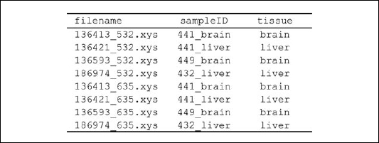
Raw data obtained from the CHARM microarrays (.xys files) can most easily be analyzed using the R/Bioconductor software environment (Gentleman et al., 2004), as normalization functions and a custom array annotation package have been made available.
There are three main components of CHARM array analysis. The first part of the analysis involves normalization. The basic measure of methylation is the log-ratio of intensities in the untreated and methyl-depleted channels. Normalization serves the dual purposes of setting the zero-methylation signal level within each array and removing the nonlinear dependence of the log-ratio (M) on the average signal intensity in the two channels (A). Loess normalization is widely used in two-color expression arrays to correct this M-A bias under the assumption that most genes are not differentially expressed (M=0) (Yang et al., 2002). However, this assumption is not appropriate when examining DNA methylation data, since many sites may be methylated and represented by positive M-values. A modified strategy involves fitting a loess regression through a subset of control probes known to represent unmethylated regions, and then applying this correction curve to all the probes on the array (Irizarry et al., 2008). The control probes are selected from CpG-free regions of the genome that are guaranteed to remain uncut by McrBC.
Following normalization, a moving window smoother is applied. The smoothed M-value at a given location is obtained by taking a weighted mean of probes within a prespecified distance of the location (Irizarry et al., 2008). A typical window size is 10 to 20 probes. This procedure significantly reduces the impact of probe-effect biases and noise on methylation estimates at the single-CpG level.
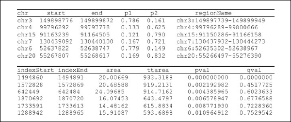
Lastly, regions with differential methylation between phenotypes are identified. For each probe, the average M-value is computed for each phenotype. Differential methylation is quantified for each pairwise tissue comparison by the difference of averaged M values (DM). Replicates are used to estimate probe-specific standard deviation (S.D.), which provide standard errors (S.E.M.) for DM. Z scores (DM/S.E.M.) are calculated, and statistically significant values (typically p < 0.001 or p < 0.005) are grouped into candidate DMR regions. A useful metric for ranking regions is the area defined as the length by average DM. In experiments with at least six biological replicates per experimental group, it is possible to calculate a statistical significance in terms of the false discovery rate (FDR) associated with each DMR. Permutation p values are generated using a null distribution of DMR areas generated by repeatedly assigning permuted group labels to samples and rerunning the DMR identification procedure. Permutation p values are then converted into q values (corresponding to FDRs) using the Bayesian procedure of Storey (2003).
Materials
qvalue (http://bioconductor.org/packages/bioc/html/qvalue.html)
Analyze raw data (.xys files) obtained from the CHARM HD2 arrays
Also see http://www.biostat.jhsph.edu/~maryee/charm for additional software details and support.
SUPPORT PROTOCOL 1
FRACTIONATION OF GENOMIC DNA BY RANDOM SHEARING
In this protocol, we describe how to randomly shear 5 µg of high-quality and high-molecular-weight genomic DNA (gDNA) from 1.5 kb to 3.0 kb using a HydroShear device (DigiLab, http://www.digilabglobal.com/). The HydroShear uses hydrodynamic forces to randomly shear gDNA to a specified size range. More specifically, the device contracts and causes the gDNA solution to pass through a 0.05-mm diameter orifice in a ruby, located within the shearing assembly. In turn, the flow rate of the solution accelerates forcing the gDNA to stretch and break (Oefner et al., 1996; Thorstenson et al., 1998). Following shearing, the DNA is equally split into two aliquots and is ready for methylation-dependent fractionation. Figure 20.1.4 provides an example of the expected distribution of DNA sizes after shearing has been performed.
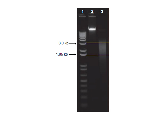
Figure 20.1.4 The expected size distribution, from 1.5 kb to 3.0 kb, of genomic DNA after shearing with a HydroShear device. We ran 500 ng of DNA on a 1% agarose gel in 1× TAE buffer for 60 min at 110 volts. Lane 1 contains a 1 Kb Plus DNA Ladder with the upper and lower arrows denoting 3.0 kb and 1.65 kb, respectively. Lane 2 contains unsheared, high-quality, high-molecular-weight genomic DNA as a reference. Lane 3 contains genomic DNA that was sheared using a standard shearing assembly on a HydroShear device. The two straight horizontal lines denote the expected size distribution of DNA.
Materials
Related posts:

Stay updated, free articles. Join our Telegram channel

Full access? Get Clinical Tree


